GC×GC: The Road Not Taken?

Some time ago, I received an email from a company producing renewable hydrocarbon oils. They were looking for a laboratory offering routine GC×GC analysis, so that they could convince potential customers that their oils are suitable for cosmetic and personal care products. They used GC-MS for characterization of the oils, but were looking to GC×GC for a much more complete picture. Unfortunately, I could not refer them to any routine laboratory that offered such services because – to the best of my knowledge – no such laboratories exist.

The antinomy of analysis

The exchange got me thinking about the paradoxical situation GC×GC finds itself in at the moment. On the one hand, most chemists now realize the true power of the technique in the analysis of complex samples. As the number of GC×GC papers continues to grow, so does the awareness of the benefits of the technique. Literature contains numerous examples of quite spectacular results obtained with GC×GC, which of course fuels further interest. Some industries, especially petroleum (1), realized quite some time ago that they could never get such detailed information on their products (in as little time) using alternative approaches – so they adopted GC×GC for routine use. Unfortunately, this is not widely publicized – perhaps because it is considered a trade secret and could provide a competitive advantage. Still, petroleum industry professionals are well aware of the power of GCxGC and often consider it to be an indispensable tool for product characterization. 

I suspect this attitude probably permeates to industries using petroleum products as raw materials (including cosmetics and personal care products), which would explain why I received the unusual request mentioned above. Other areas where GC×GC plays a very important role include metabolomics (2) and environmental analysis, the latter being the first to adopt an official GC×GC-based analytical method (3). Overall, for many analytical scientists, GC×GC is now the go-to technique for dealing with very complex samples.

Which brings me to the other side of the coin: if GC×GC is now recognized as being a very powerful technique, why is it not used routinely by anyone outside of a relatively narrow cluster of research laboratories and industries? Why can’t someone outside of this cluster simply send a sample to a commercial laboratory to have it characterized by GC×GC? As practitioners of the technique, we should be asking ourselves why there is so clearly a disconnect between the great promise of the technique and its wider adoption. Having thought about this question quite extensively, I would like to share some of my own conclusions, with the explicit understanding that these may not be shared by all.  

Intricate beginnings 

To me, the elephant in the room is the perceived (or real) complexity of the technique. GC is relatively easy to explain to students, and people who use it typically have a reasonably good grasp of the technique. Generally speaking, GC is easy to learn. You install a typical 30 m x 0.25 mm ID x 0.25 μm d_f column in a GC oven, inject a sample at a relatively low temperature, then program the oven to heat up to a certain final temperature that should be high enough to allow all sample components to elute from the column, but not so high that the stationary phase would be destroyed. If some components fail to separate, one can play with the temperature program and/or carrier gas flow rate. If that does not help, you can try a longer column or switch to a different column – and that’s about it.
 

Contrast that with GC×GC, where one has to choose not one, but two columns and decide on their geometries. Should I use a 30 m or 60 m column in the first dimension (¹D)? Should it be polar or nonpolar? What column length should I use in the second dimension (²D)? What should be its internal diameter? The stationary phase? Most users look for generic methods as the starting point to method development. A typical configuration these days would include a nonpolar column in ¹D, and a semipolar or polar one in ²D, but that is not always the best combination. One then needs to choose the modulator. In the early days, the choices were rather limited, as cryogenic modulators were the only ones commercially available. The picture is definitely more complicated these days (4). Though cryogenic modulators still dominate, they now face serious competition from thermal and (in particular) various flow modulation platforms (see Figure 1 for selected examples). Each modulator type has its strengths and weaknesses, but none can claim that it is definitely the best for all applications. 

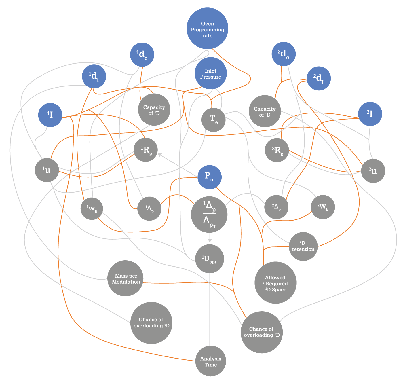
Once the modulator is chosen, the user faces method development. Right from the beginning, it's more complicated than in standard GC. In addition to the parameters that are normally adjusted in a one-dimensional GC method, the user has to decide on the length of the modulation period and the secondary oven temperature offset (if available). Further to this, certain parameters specific to a given modulator platform must be selected. If this were the end of the story, an average GC user would be able to learn how to develop a GC×GC method quite quickly. However, things get more complicated still because of the mutual dependence of many parameters in GC×GC – as we tried to illustrate with the now quite (in)famous spaghetti diagram (see Figure 2) published originally in 2007 (5) and then reprinted in an improved version in 2012 (6). For example, changing the oven temperature ramp changes the elution temperature of an analyte, which in turn affects its retention in ²D. It may also change the ¹D peak width, which will affect the number of times a given ¹D peak is sampled, and that in turn affects peak resolution and method sensitivity. For an inexperienced user, this may quickly lead to confusion – and lots of hand-wringing!
 

The chromatogram and software

Suppose, though, that our hypothetical new user successfully navigates the GC×GC method development waters and is now prepared to get down to some real analyses. Unfortunately, there are further obstacles awaiting them! Indeed, acquiring the data is just the first step – getting the required information from the raw data is a whole new ball game. 

In ¹D GC, the chromatogram is a simple plot of signal intensity as a function of time. Peaks have (more or less) Gaussian shapes, and the peak area is proportional to the amount of the analyte. Problems mostly arise due to incomplete peak resolution and the uncertainties related to determining the start and stop of a peak, especially when it is asymmetrical. Over the many years of development, manufacturers of GC instrumentation managed to develop pretty robust tools that can adequately handle most situations, and manual intervention is rarely required (and generally avoided). The procedures are more or less standardized by now, hence users do not have to worry that a different software package will handle their data differently. 

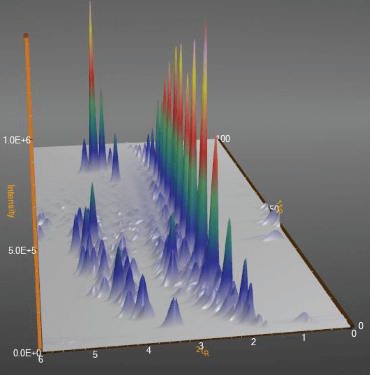
Unfortunately, this is not yet the case with GC×GC. A raw GC×GC chromatogram does not differ from the one obtained in ¹D GC – it is also a plot of signal intensity as a function of time. The two-dimensional structure of the data has to be brought out through data processing. The basics are quite simple and are the same for all software packages – the raw chromatogram is “cut” into segments corresponding to the individual modulation periods, which are then placed side-by-side to produce a two-dimensional map on which signal intensity is coded with different colors, or a three-dimensional representation that can be easily manipulated on the computer screen (and which produces the pretty pictures so popular in GC×GC publications – see Figure 3). 

What happens next, though, very much depends on the software package being used. When quantitation is required, the areas of peaks of a given analyte in the individual modulation periods need to be added to yield the total area of the peak (which should be the same, in principle, as the corresponding ¹D peak area). However, this requires that the peaks belonging to a given analyte in the consecutive modulation periods (“slices”) be properly identified. With non-selective detectors, the identification can only be based on ²D retention times. 

However, this task is not straightforward, as every consecutive ²D chromatogram is developed at progressively higher temperature in a temperature-programmed run, hence the ²D retention times become shorter in each consecutive “slice.” If a peak is well resolved, symmetrical, and sampled the recommended two-to-three times, this is typically not an issue and proper reconstruction of the total peak area is quite straightforward. However, tailing peaks are much more difficult to deal with. The progressively shorter ²D retention times produce the characteristic banana-shaped profiles, and most software packages have problems with accurate assignment of all the component slices in which the tail of a given peak is still present. The job is a little easier when MS is used for detection, but the noise that inevitably creeps into the spectra when the tail becomes small can throw these software packages off as well. 

To complicate life even further, different software packages deal with the integration differently. Some stick to integration of the component peak areas in the raw signal and simple summation of them; others might resort to summing of peak heights to reduce the computational requirements. Yet another solution is to try to “reconstruct” the shape of the peak in three dimensions and assign a volume to it rather than an area. All of these approaches have their benefits and shortcomings, but the net result is that the same raw data processed with different software packages might not produce identical results, as recently described by Weggler et al (7). 

It’s not all bad… 

If you have reached this point of my deliberations, you may wonder whether my purpose is to discourage people from using GC×GC. Let me assure you that this is not the case – in fact the opposite is true. What I am trying to do is figure out the best ways to help new and inexperienced users navigate choppy GC×GC waters, and to finally bring GCxGC where it belongs – into the mainstream!

First and foremost, I believe education is the foundation of future success. GC×GC courses offered at different conferences can be a great introduction to the technique, but due to their (necessarily) short duration, future users will not learn how to navigate GC×GC waters effortlessly. Some instrument manufacturers offer great training courses, but they are limited to their customers only. I would love to see manufacturers and leading experts in the field joining forces to organize in-depth training courses, including hands-on experience, that are open to everybody. I am not sure of the best way to accomplish this, but as they say, “where there’s a will, there’s a way.”

For industry to widely adopt the technique, we need robust, reliable, and fully validated turn-key solutions. As much as my researcher’s gut hates the “black box” concept, I believe this is exactly what the industry needs. Some manufacturers are trying to do it already, and that is very encouraging. 

Conquering the commercial laboratories is a much taller order, because official methods are desperately needed. No commercial laboratory will invest a single penny into a technology that produces results that will not be accepted by regulatory agencies or are not defensible in the court of law. The task of changing this falls on the shoulders of both the manufacturers and the users of the technique. If you have developed a fantastic method that solves a real problem, maybe you should think about taking it a step further and turning it into an official method. It may be lot of work, but it would be a great service to the GC×GC community – and, ultimately, society as a whole. 

Finally, there is certainly room for budding entrepreneurs to open dedicated GC×GC laboratories that could handle odd requests (like the one that inspired this feature), routine analyses, and consulting services. With a little marketing, I am quite confident they would not sit idle.

I have to emphasize once again that these are my personal opinions; the true path to bringing GC×GC into the mainstream might be completely different. If you have different ideas, I would love to hear them. Maybe they will form the basis for a follow-up article!

References

- (1) BJ Pollo et al., “The impact of comprehensive two-dimensional gas chromatography on oil & gas analysis: Recent advances and applications in petroleum industry”, TrAC Trends Anal Chem, 105, 202 (2018). DOI: https://doi.org/10.1016/j.trac.2018.05.007
- (2) EA Higgins Keppler et al., “Advances in the application of comprehensive two-dimensional gas chromatography in metabolomics,” TrAC Trends Anal Chem, 109, 275 (2018). DOI: 10.1016/j.trac.2018.10.015
- (3) Muscalu, E. Reiner, S. Liss, T. Chen, G. Ladwig, D. Morse, “A routine accredited method for the analysis of polychlorinated biphenyls, organochlorine pesticides, chlorobenzenes and screening of other halogenated organics in soil, sediment and sludge by GCxGC-μECD”, Anal. Bioanal. Chem. 401 (2011) 2403-2413. DOI: https://doi.org/10.1007/s00216-011-5114-0
- (4) HD Bahaghighat et al., “Recent advances in modulator technology for comprehensive two dimensional gas chromatography,” TrAC Trends Anal Chem 113, 379 (2019). DOI: https://doi.org/10.1016/j.trac.2018.04.016
- (5) J Harynuk and T Górecki, “Experimental variables in GCxGC: A complex interplay,” American Laboratory News, 39, 36 (2007).
- (6) A Mostafa et al., “Optimization aspects of comprehensive two-dimensional gas chromatography,” J Chromatogr A, 1255, 38 (2012). DOI: https://doi.org/10.1016/j.chroma.2012.02.064
- (7) BA Weggler, LM. Dubois, N Gawlitta, T Gröger, J Moncur, L Mondello, S Reichenbach, P Tranchida, Z Zhao, R Zimmermann, M Zoccali, J-F Focant, “A unique data analysis framework and open source benchmark data set for the analysis of comprehensive two-dimensional gas chromatography software, Journal of Chromatography A, in press (2020). DOI: https://doi.org/10.1016/j.chroma.2020.461721